Velocity Vectors: Secondary Solutions!

Hello, again! Encouraged by my sudden lack in homework and with interest in the problem at an all-time high, I decided to write a Part 2 about the idea of velocity vectors immediately! 😀
If you haven’t read the original post, I would highly suggest doing so first: https://elytraflight.com/2021/05/17/velocity-vectors-circles-and-calculus/ The main objective of this post is to go over two different approaches to the same problem, and to discuss their benefits and drawbacks. For now, however, let’s do this!

First, let’s reiterate the problem:

“A particle moves along a curve so that its position vector and velocity vector are perpendicular at all times. If the particle passes through the point (4, 3), what is the equation of the curve?”

Solution 2

In the previous post, we used a solution involving linear algebra, but who wants linear algebra? After all, linear algebra is just a bunch of funny number magic, right?

So, we decide to attack the problem an alternative way!
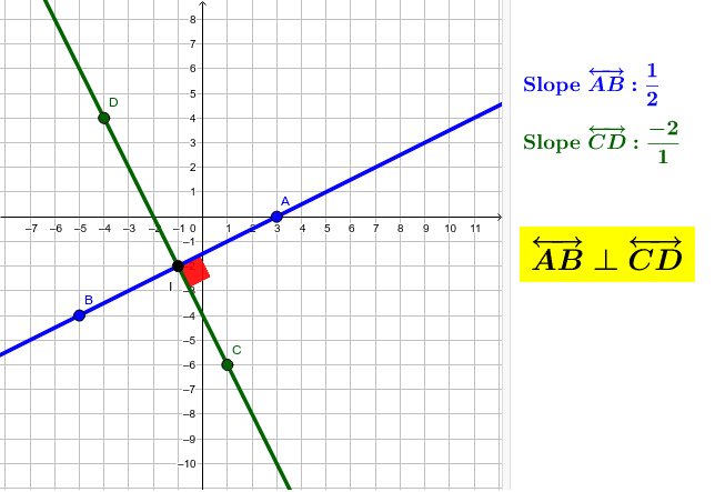
Consider what it means for two lines to be perpendicular. With two lines in the form of y = mx + b, the slopes have to be negative reciprocals of each other (e.g. 1/2 and -2 in the diagram below).

What does this mean for our problem? Let’s recall our position vector s(t) = (x(t), y(t)). The “slope” of our position vector, in this case, can be found with the general “rise over run” technique: m = (y-0)/(x-0) = y/x.

However, as we mentioned before, our velocity vector, v(t) = (x'(t), y'(t)), is perpendicular to the position vector! Thus, we know that the “slope” of our velocity vector, y'(t)/x'(t), is the negative reciprocal of y/x, which happens to be -x/y. So, this is what we end up with:

However, the second equality is more than just an equation; it’s a differential equation! A differential equation that we have the tools to solve, as a matter of fact!

Our first step is to separate the variables. We can move the dx to the right side and the y to the left side, to arrive at an equation as follows:

Time to integrate both sides!

Voila! We have arrived at the exact same answer as we did with the other method. Just like last time, we can plug in a specific case for x and y to find a specific case. Beautiful! 😀

Solution 3

And, last but not least, we have our final solution! Suppose we are still slightly suspicious of dot products, but we’re willing to give parametric functions (and some inefficient but cool techniques) a chance. Edit: After researching this solution a bit more, I realized that this solution gets crazy quite quickly. Buckle up!

Jumping right in, we reintroduce our vectors s(t) = (x(t), y(t)), and v(t) = (x'(t), y'(t)). However, this time we have a twist. This time, we don’t end up removing t to get a general form of the circle equation in terms of x and y. No; this time, we dig even deeper. What we intend to do today is find both x(t) and y(t) in general form.

In the above example, we see that we are taking advantage of a very important characteristic of perpendicular vectors. We take the x position, making it negative and multiplying by some constant a (as we do not want to assume that the velocity vector is the same magnitude as the position vector).

Note that we are multiplying by a constant value a. This will be important at the end.
So here’s the two equations we have so far:

x'(t) = a y(t)
y'(t) = -a x(t)

Let’s start by manipulating the first equation, moving a to the other side.
y(t) = x'(t)/a
Now, we take the derivative of both sides:
y'(t) = x”(t)/a
We now have two different formulas for y'(t). Let’s set them equal to each other!
x”(t)/a = -a x(t)
x”(t) = -a²x(t)

We now have a seemingly simple differential equation, with the second derivative in terms of the original function. However, we can’t just integrate, as that would leave us with a first derivative and some unruly antiderivative of x(t).
Our options are running out! With no options left, we have no choice but to put on our LaTeX gloves (hahaha I’m hilarious) and set out on a journey into Laplace Land.

Ahh, sunlight fills our eyes, and fresh air enters our lungs. At last, after all that pain and effort, here we are with our two final, completely general equations for x(t) and y(t):

And, you know what this means! If we find x²+y², it will equal some constant not in terms of t, which is the radius of our new circle squared. Granted, this newly-found radius of the circle will be in terms of the given values for x(0), x'(0), and a, but that is to be expected.

Some of the incredibly astute may recall previously experimenting with piecewise functions, and how these trig functions are by no means the only two functions that can produce circles. For instance, something as simple as

can follow the path of a (semi)circle within its domain. Furthermore, parametric functions like these also satisfy the property of having position vectors and velocity vectors being perpendicular, since x²+y²=R; in the previous solutions, we demonstrated that this is enough to conclude that the velocity vector is always tangent to the position vector in such a scenario. However, our very complex-looking trigonometric formula up above is incredibly special, in that it is the only general case parametric function out there whose value for “a” stays constant everywhere. In other cases, such as x(t) = t, the two vectors are perpendicular, but the ratio in magnitudes varies wildly depending on t. In our above case, however, a stays constant. Everywhere.

If one is skeptical, we can test these formulas, and demonstrate that for any value of x(0) and x'(0) and a, the difference in magnitudes of the position and velocity vectors will indeed still be a, and by taking the derivatives of the formulas for x(t) and y(t) show that the formulas do indeed work out with what they should be. A true mathematical miracle.

This concludes the third and final solution to this amazing problem. What a crazy experience! This took me about 10 hours of work to finish, between the three different solutions. I now intend to rest for the time being.

It’s been an honor to have all of you readers along on this journey. As always, until we meet again, best wishes, and happy exploring!

– Ely